SOT를 측정하는데 있어 가장 대중적으로 알려진 방법으로 haromic Hall voltage measurements method가 있습니다.(자세한 정성적 설명 및 발전 단계는 해당 글에서 참고 할 수 있으므로 생략하겠습니다) 하지만 정량적인 공식에 대해서는 (물론 굳이 할 필요는 없지만) 증명을 풀어 설명하는 글이 충분치 않고 그저 최종 공식이 떡하니 제시되어 있는 경우가 허다합니다.
이에 단계 단계 어떤 과정을 거치고 어떤 가정을 하는지 자세히 설명한 thesis가 있어 재정리 겸 글을 올립니다. 글에 있는 모든 공식과 그림 자료는 해당 thesis에서 가져왔습니다.
원문: Mechanism of spin-orbit torques in platinum oxide systems - Jayshankar Nath
우선 가장 기본부터 시작하자. 주파수 $\omega$를 가지는 교류 전류가 채널에 흐를 때, 측정되는 transverse Hall voltage는 다음과 같다.

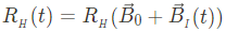
여기서 Hall resistance $ R_{_H}(t)$는 다음과 같이 구성된다.
- static : $\vec{B}_{0}$, The sum of external anisotropy and demagnetizing fields.
- dynamic : $\vec{B}_{_I}=\vec{B}_{DL}+\vec{B}_{FL}-\vec{B}_{Oe}$, The sum of current-induced fields.
하지만 실제 환경에서는, 열텀 $ R_{_T}cos2\omega t $ 가 자화의 equilibrium position에 영향을 끼쳐 Hall resistance는 아래와 같이 변한다.

열텀으로 인해 바뀐 새로운 equilibrium position 주변에서 Taylor series expansion을 진행하면

그러면, Hall voltage는 아래와 같다.

좀 더 풀어서 쓰면


정리하면

where
- $R_{H}^{0}$ : the zeroth harmonic components of the Hall resistance
- $R_{H}^{f}$ : the first harmonic components of the Hall resistance
- $R_{H}^{2f}$ : the second harmonic components of the Hall resistance
- $R_{H}^{3f}$ : the third harmonic components of the Hall resistance
위에서 추가한 열에 의한 equilibirium point의 이동은 정류 전압으로 발현되기에 무시할 수 있다. 그러므로 ,

Zeroth, first, second harmonic 중 first harmonic이 자화의 equilibrium position을 나타내며, 아래와 같이 쓸 수 있다.

Second harmonic은 전류에 의해 유도되는 자화의 변화를 나타내며, 구좌표계에서 아래와 같이 전개시킬 수 있다.


가정1: Uniaxial anisotropy contribution이 매우 작다고 무시하자. 이 경우, 자화에 가해지는 current-induced field의 효과는 polar contribution과 azimuthal contribution으로 나눠질 수 있다.


이렇게 나눠질 경우 current-induced field contribution은 외부장 $ \vec{B}_{ext} $에 의한 것과 정량적 비교가 가능해진다.구좌표계의 differential element를 보면

그러면 differential field는 다음과 같이 쓸 수 있다.

이 항이 전류나 외부장을 약간 변화시킬때 magnetization에 영향을 끼치는 field이다.
가정2: 우리가 수행하는 angular scan은 x-y plane, y-z plane에 국한된다. 그러므로 magnetization의 $\theta_{B}$ ($\phi_{B}$)성분에 대해서 볼 때는 external differential field의 $\phi_{B}$ ($\theta_{B}$) 성분은 무시해도 된다.

Angular scan 중에, 우리는 외부 장을 고정시킨다. 그러므로 radial 방향으로는 $ d B_{ext}=0 $이 성립한다. 또한
가정3: SOT에 의해 발생하는 radial axis 방향의 magneitzation 변화는 무시한다.
$\theta$방향으로의 differential field는 다음과 같다.

또한 이 field를 magnetization vector로 projection 했을 때는 다음과 같을 것이다. (Figure 1 참고)


위와 유사하게, $\phi$ axis 방향으로는

그리고 이 field 역시 magnetization vector로 projection 하면


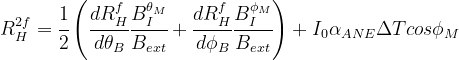
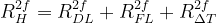
위에서 구한 식들을 second harmonic resistance 공식에 대입시키면

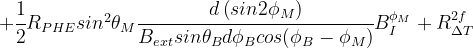
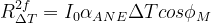
위의 식에서 $R_{\Delta T}^{2f}$ 항은 샘플에 전류를 주입할때 발생하는 thermal gradient에 의한 second harmonic resistance를 나타낸다. 일반적으로, 전류를 주입한 방향에 수직 방향으로 thermal gradient가 발생하고, 이로 인해 ANE를 유발한다. 우리는 Hall bar가 아닌 Hall cross를 이용하여 lateral 방향의 thermal gradient를 최소화 시켰다.
하지만, 노광공정에서 조금만 misalignment가 발생하면 lateral gradient가 발생할 수도 있다. 이 thermo-electric 신호는 zeroth order와 second order에 추가 되며, 실험적으로 아래와 같은 경향을 보인다.
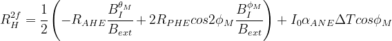
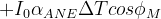
우리의 연구주제인 metallic film에서는 이 thermo-electric signal의 주된 contribution은 ANE이며, 아래와 같이 쓰여진다. ($\alpha_{ANE}$는 ANE coefficien이다)

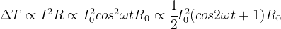
이를 반영한 식을 대입하여 다시 second harmonic resistance 공식을 쓰면
Harmonic Hall voltage measurement가 대부분 in-plane anisotropy를 가지는 샘플들에 대해서 이루어지므로, 대부분이 in-plane angle scan(x-y plane scan)을 진행한다. we mostly utilize in-plane angle scans, wherein we apply a constant rotating field in the plane of the film in Figure 2.
(Peprpendicular anisotropy를 가지는 샘플에서도 이 방법은 활용될 수 있다, with an anisotropy field much lower than that of the maximum applicable external field).
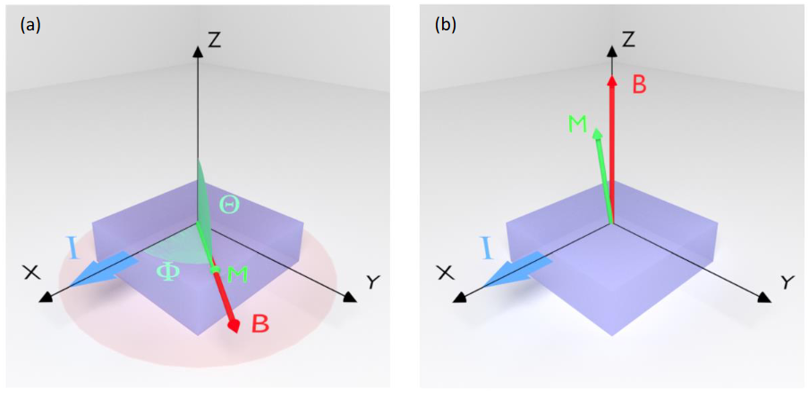
In-plane angle scan의 경우, field가 film의 plane에서만 회전하므로, $\theta $는 $\cfrac{pi}{2}$로 고정된 값을 가진다.
가정4: 측정에 쓰이는 샘플이 in-plane anisotropy를 가짐과 동시에 위에 가정했듯이 매우 약한 uniaxial in-plane anisotropy를 가지므로, 우리는 magnetization이 external field의 방향에 동기화 될 것으로 예상할 수 있다.
그러므로 다음과 같이 쓸 수 있다.
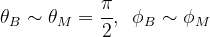
이 constraints를 이용하여 위의 식에 대입하면

Planar Hall coefficient와 anomalous Hall coefficient는 first harmonic response에서 구할 수 있음을 기억하자.
This can be computed, by once again considering, $\theta_{B} \sim \theta_{M} = \cfrac{\pi}{2}, \; \phi_{B} \sim \phi_{M})$, as follows

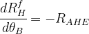
For AHE term, 미분 변수를 보면 알겠지만 y-z plane scan이 필요하다.
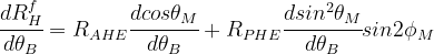

At $\theta_{M}= \cfrac{\pi}{2}$,

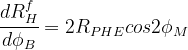
For PHE term, 미분 변수를 보면 알겠지만 x-y plane scan이 필요하다.
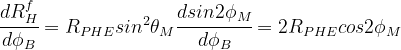
Then we can write the equation
as like
where
더 나아가기 위해, 인가되는 전류에 의해 발생하는 torque의 symmetry를 한번 생각해보자. 레퍼런스로 일반적인 Pt/Co/AlOx system을 이용하면, 우리는 orthogonal torques, DLT, FLT의 부호를 고정시킬 수 있다. (Figure 3 참고)
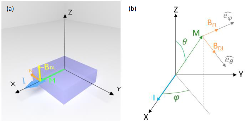
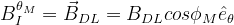
구 좌표계에서 DL field는 아래와 같이 쓸 수 있다.


x-y scan이므로, $\theta_{M}=\cfrac{\pi}{2}$ 임을 이용하면

비슷한 방식으로, FL field 역시 구 좌표계에서 나타낼 수 있다.


정리하면
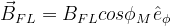
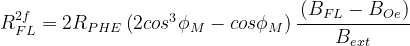
위에서 구한 구좌표계에서의 DL field와 FL field를 보면, DL field는 $\theta$축과 평행한 방향으로 magnetization에 작용하며, FL field는 $\phi$축과 평행한 방향으로 작용함을 알 수 있다. 그러면 지난 번에 구한 $B_{I}^{\theta_{M}}$, $B_{I}^{\phi_{M}}$은 아래와 같이 쓸 수 있다.

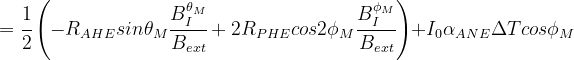
이제 이 식들을 위 어딘가에 있는 second harmonic resistance 공식에 집어 넣으면


보다시피, second harmonic resistance는 DLT, FLT, 그리고 thermo-electric effect에 의한 torque까지 총 3개의 factor를 포함하고 있다. 이 3개의 factor들에 대해 second harmonic resistance를 정리해보자.
We define
Then


Thermal effect로부터 DLT와 FLT를 분리시키기 위해서는, 식에서 보이는 것 처럼 $B_{ext}$ dependence를 고려해야 한다. 보다시피 DL field와 FL field는 각각 $B_{ext}$에 반비례하지만, thermal effect는 independent하다. 또한,
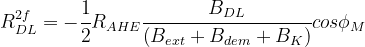
자화에 작용하는 static field도 고려해야 한다. 이는 앞에서도 언급한 anisotropy field와 demagnetization field이다. 이 항들은 DL field와 FL field에 대해 정량적으로 정확한 값을 구할 때 필요하다.
우선 DL field와 관련된 값들을 보자. DL SOT는 자화가 sample의 out of plane 방향으로 움직이게끔 유도하며, 이를 식으로 나타내면, $\cfrac{dR_{_H}^{f}}{d\theta_{_B}}$ 이다. 이 항은 in-plane external field에 역으로 작용한다고 볼 수 있다. 또한 anisotropy field와 demagnetization field 역시 자화를 샘플의 plane에 있게끔 DL field에 역으로 작용한다.
FL field 관련 하여서는, FL SOT는 샘플의 plane 내에서 magnetization을 plane에서 밀어내는(더 빠르게 회전하도록) 효과를 내며 이는 in-plane external field와 in-plane uniaxial anisotropy에 역작용으로써 작용한다.
하지만 앞에서 가정했듯이, 우리가 현재 고려하는 샘플은 in-plane uniaxial anisotropy가 매우 작은 값을가지며 이 항은 무시해도 된다.
However, as our samples have negligible in-plane uniaxial anisotropy, this term can be ignored.
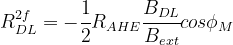
그러므로, 위의 방정식들을 다시 쓰면, $R_{_{DL}}^{2f}$, $R_{_{FL}}^{2f}$, and $R_{_{\Delta T}}^{2f}$는 아래와 같이 각각 쓸 수 있다.
이를 통해 성공적으로 DL term, FL term, thermal term을 분리시켰다.
이후의 DL field, FL field, thermal coefficient는 위의 식을 fitting하여 얻을 수 있을 것이다.
정리해보자.
우선 우리가 한 가정은 다음과 같다.
1: Uniaxial anisotropy contribution이 매우 작다고 무시하자. 이 경우, 자화에 가해지는 current-induced field의 효과는 polar contribution과 azimuthal contribution으로 나눠질 수 있다.
2: 우리가 수행하는 angular scan은 x-y plane, y-z plane에 국한된다. 그러므로 magnetization의 $\theta_{B}$ ($\phi_{B}$)성분에 대해서 볼 때는 external differential field의 $\phi_{B}$ ($\theta_{B}$) 성분은 무시해도 된다.
3: SOT에 의해 발생하는 radial axis 방향의 magneitzation 변화는 무시한다.
4: 측정에 쓰이는 샘플이 in-plane anisotropy를 가짐과 동시에 위에 가정했듯이 매우 약한 uniaxial in-plane anisotropy를 가지므로, 우리는 magnetization이 external field의 방향에 동기화 될 것으로 예상할 수 있다.
'Other Topics' 카테고리의 다른 글
| Wavepacket (파속) in Quantum Mechanics (0) | 2023.03.13 |
|---|---|
| Eigenstates의 확률 진폭의 분포를 나타내는 두가지 방법 (1) | 2023.03.13 |
| (작성중) 밸리트로닉스 (Valleytronics) (1) | 2023.03.07 |
| (작성중) 오비트로닉스 (Orbitronics) (0) | 2022.08.29 |
| 교환 상호작용 (Exchange interaction) (0) | 2021.05.27 |


댓글